The Musk Effect: Quantifying Elon’s Impact on Tesla's Stock
How does public sentiment toward Elon Musk affect Tesla’s stock price? At ForecastOS, we built exactly the tool to determine this; enter ForecastOS Hivemind.
In this blog post, we use Hivemind to create a time series factor based on changes in aggregate sentiment about whether Elon Musk is a genius. We calculate how this factor correlates with Tesla’s forward stock returns and use it as a signal in a single-stock long/short trading strategy.
Agenda
- What is ForecastOS Hivemind?
- Hivemind Poll: "Is Elon Musk a Genius?"
- Elon - TSLA Correlation
- "Is Elon Musk a Genius?" Trading Strategy
- Build Your Own Predictive Signals With Hivemind
- Full Code
1. What is ForecastOS Hivemind?
ForecastOS Hivemind is an AI-powered platform that continuously ingests data from top media and financial sources. It allows you to create time series factors from unstructured data using generative AI.
If you can identify a topic that influences a stock’s value, Hivemind can track consensus over time and convert it into a signal with alpha potential.
Hivemind can also identify emerging trends and generate company-level risk exposures. For example, it recently flagged the Iran strike days before it occurred and identified the stocks likely to be positively or negatively impacted.
Generating Tariff Exposures with ForecastOS Hivemind
Read more about Hivemind here:
AI Analyzes the Internet: Elon Musk’s Genius Rating Tanks. Is Tesla Stock Next?
Hivemind Trends: April 27 to May 4
2. Hivemind Poll: "Is Elon Musk a Genius?"
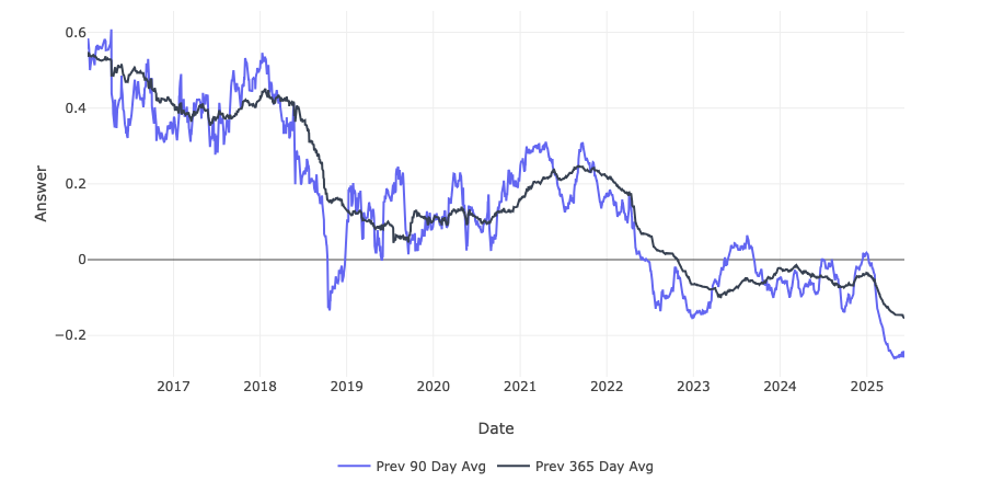
73,315 mentions of Elon Musk were evaluated to assess whether speakers agreed with the statement, "Elon Musk is a genius." Responses generated by AI were scored as 1 for yes, 0 for neutral or no opinion, and -1 for no. Rolling averages over 90 and 365 days were then calculated to produce the graph shown below.
3. Elon - TSLA Correlation
Using 90-day rolling average “Elon Musk is a genius” sentiment and Tesla stock price data from ForecastOS FeatureHub, we examined if sentiment shifts were correlated with forward stock returns.
| Sentiment Change Window | Forward Return Period | Pearson Corr (P-Value) |
|---|---|---|
| 1-day | 5-day | 0.0234 (0.17) |
| 30-day | 5-day | 0.0627 (0.00026) |
The 1-day sentiment change isn’t statistically significant, likely due to higher noise / volatility at that time horizon. The 30-day change, however, shows strong statistical significance!
4. "Is Elon Musk a Genius?" Trading Strategy
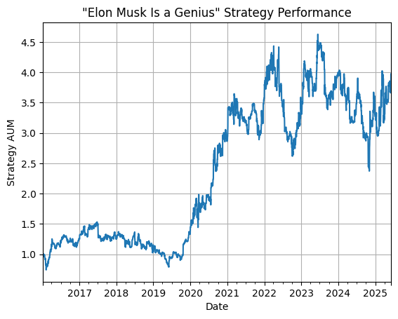
Given the positive correlation between changes in Elon Musk genius sentiment and Tesla stock returns, we tested a simple trading strategy using sentiment changes as a signal.
The strategy goes long when sentiment rises and short when it falls. Below is the performance graph for the strategy.
To show our performance is not simply due to the percentage of positive and negative positions, especially since Tesla’s price rose ~30x over the backtest period, we benchmarked against a randomized strategy. This strategy takes random positions with the same positive and negative ratio as our sentiment factor. Below is the performance graph for the randomized strategy.
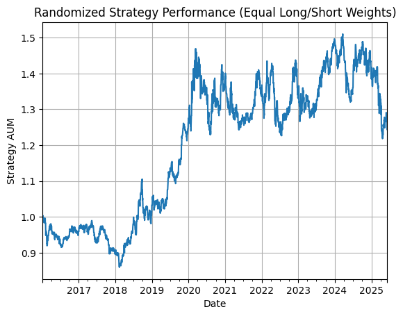
The strategy that uses our sentiment factor outperforms the randomized version by roughly 3x, confirming the predictive value of our sentiment signal.
While we wouldn’t advocate running this strategy on its own, especially due to its high volatility, turnover, and associated trading costs, it’s an example of a great addition / input to a wider fundamental or quantitative investment strategy!
5. Build Your Own Predictive Signals With Hivemind
This is just one example of how Hivemind can be used to easily create forward-predictive signals that generate alpha. With Hivemind, any topic can become a time series factor, providing you with new, customizable risk and alpha inputs.
If you want to build your own signals, such as risk exposures to tariffs or recession likelihood sentiment, Hivemind makes it easy. Click below to start your free trial today!
6. Full Code
import pandas as pd
import os, forecastos as fos
import numpy as np
from scipy.stats import pearsonr

# -------------------------------------------------------
# 1. Get Elon sentiment data
# -------------------------------------------------------

# Poll results generated by Hivemind
df_elon_sentiment = pd.read_csv('./elon_poll.csv')
df_elon_sentiment['episode_date'] = pd.to_datetime(df_elon_sentiment['episode_date'])

# Create a full date range from min to max date
full_range = pd.date_range(
  start=df_elon_sentiment['episode_date'].min(),
  end=df_elon_sentiment['episode_date'].max(),
  freq='D'
)

# Reindex the DataFrame with the full date range
df_full = df_elon_sentiment.set_index('episode_date').reindex(full_range)

# Rename the index to 'episode_date'
df_full.index.name = 'episode_date'

# Forward fill the rolling_avg column
df_full['rolling_avg'] = df_full['rolling_avg'].ffill()

# Reset index
df_full = df_full.reset_index()

# Shift by 1 day to avoid lookahead
# --> (sentiment comes in over entire day for datetime, using open to open returns)
df_full['rolling_avg'] = df_full['rolling_avg'].shift(1)

# Update sentiment data to include all dates
df_elon_sentiment = df_full

# Calculate changes in sentiment over different time windows
df_elon_sentiment["rolling_avg_prev_1d_diff"] = df_elon_sentiment["rolling_avg"] - df_elon_sentiment["rolling_avg"].shift(1)
df_elon_sentiment["rolling_avg_prev_2d_diff"] = df_elon_sentiment["rolling_avg"] - df_elon_sentiment["rolling_avg"].shift(2)
df_elon_sentiment["rolling_avg_prev_3d_diff"] = df_elon_sentiment["rolling_avg"] - df_elon_sentiment["rolling_avg"].shift(3)
df_elon_sentiment["rolling_avg_prev_4d_diff"] = df_elon_sentiment["rolling_avg"] - df_elon_sentiment["rolling_avg"].shift(4)
df_elon_sentiment["rolling_avg_prev_5d_diff"] = df_elon_sentiment["rolling_avg"] - df_elon_sentiment["rolling_avg"].shift(5)
df_elon_sentiment["rolling_avg_prev_10d_diff"] = df_elon_sentiment["rolling_avg"] - df_elon_sentiment["rolling_avg"].shift(10)
df_elon_sentiment["rolling_avg_prev_30d_diff"] = df_elon_sentiment["rolling_avg"] - df_elon_sentiment["rolling_avg"].shift(30)
df_elon_sentiment["rolling_avg_prev_90d_diff"] = df_elon_sentiment["rolling_avg"] - df_elon_sentiment["rolling_avg"].shift(90)

df_elon_sentiment = df_elon_sentiment.rename(columns={"episode_date": "datetime"})
df_elon_sentiment['datetime'] = pd.to_datetime(df_elon_sentiment['datetime'])
df_elon_sentiment["ticker"] = 'TSLA' + '-US'

# -------------------------------------------------------
# 2. Join ticker mapping and returns data from FeatureHub
# -------------------------------------------------------

fos.api_key = os.environ.get("FORECASTOS_API_KEY_PROD")

# Ticker mapping data
df_id_mapping = fos.Feature.get(
  "79f61521-381e-4606-8020-7a9bc3130260"
).get_df().rename(columns={"value": "ticker"})

df_elon_sentiment = df_elon_sentiment.merge(df_id_mapping, on='ticker', how='left')
df_elon_sentiment['ticker'] = df_elon_sentiment['ticker'].str[:-3]

# Merge 5d returns data into df
df_prev_5d_return = fos.Feature.get(
  "8700c7c9-4d14-400b-a27b-93605d3eadbf"
).get_df()

df = df_elon_sentiment.merge(df_prev_5d_return, on=['id', 'datetime'], how='left').rename(columns={
    "value": "prev_5d_return"
})

# Merge 1d returns data into df
df_prev_1d_return = fos.Feature.get(
  "ea4d2557-7f8f-476b-b4d3-55917a941bb5"
).get_df()

df = df.merge(df_prev_1d_return, on=['id', 'datetime'], how='left').rename(columns={
    "value": "prev_1d_return"
})

df['prev_5d_return'] = df['prev_5d_return'].fillna(0)
df['fwd_5d_return'] = df['prev_5d_return'].shift(-5)
df['prev_1d_return'] = df['prev_1d_return'].fillna(0)
df['fwd_1d_return'] = df['prev_1d_return'].shift(-1)

df = df.dropna(subset=['rolling_avg_prev_2d_diff', 'fwd_5d_return', 'fwd_1d_return'])

# -------------------------------------------------------
# 3. Correlations
# -------------------------------------------------------

# --- 1 day sentiment diff correlation to returns --- #

# Drop rows with NaNs in either column
clean_df = df[['rolling_avg_prev_1d_diff', 'fwd_5d_return']].dropna()

# Compute correlation coefficient and p-value
r, p_value = pearsonr(clean_df['rolling_avg_prev_1d_diff'], clean_df['fwd_5d_return'])

print(f"Correlation coefficient (r): {r:.4f}")
print(f"P-value: {p_value:.4e}")

# --- 30 day sentiment diff correlation to returns --- #

# Drop rows with NaNs in either column
clean_df = df[['rolling_avg_prev_30d_diff', 'fwd_5d_return']].dropna()

# Compute correlation coefficient and p-value
r, p_value = pearsonr(clean_df['rolling_avg_prev_30d_diff'], clean_df['fwd_5d_return'])

print(f"Correlation coefficient (r): {r:.4f}")
print(f"P-value: {p_value:.4e}")
# -------------------------------------------------------
# 4. Simple strategy backtest
# -------------------------------------------------------

df['position'] = np.where(df['rolling_avg_prev_1d_diff'] >= 0, 0.2, -0.2)
df['position_rolling_sum_5'] = df['position'].rolling(window=5).sum()
df['strategy_return_fwd_1d'] = df["position_rolling_sum_5"] * df["fwd_1d_return"]
df['strategy_aum'] = (df['strategy_return_fwd_1d'] + 1).cumprod()

df.set_index('datetime')['strategy_aum'].plot(title='"Elon Musk Is a Genius" Strategy Performance', xlabel='Date', ylabel='Strategy AUM', grid=True)
# --------------------------------------------------------------------
# 5. Backtest with same amount negative/positive positions, but random
# --------------------------------------------------------------------

percent_negative = (df["fwd_1d_return"] < 0).mean() * 100
percent_postive = (df["fwd_1d_return"] >= 0).mean() * 100

position_negative_pos = (df["position_rolling_sum_5"] < 0).mean() * 100
position_positive_pos = (df["position_rolling_sum_5"] >= 0).mean() * 100

n = len(df)
n_neg = int(round(position_negative_pos / 100 * n))
n_pos = n - n_neg  # ensures sum to n

# Create the values
values = np.array([-0.2] * n_neg + [0.2] * n_pos)

# Shuffle the values to randomize their positions
np.random.seed(42)
np.random.shuffle(values)

# Add as a new column
df['position_random'] = values
df['strategy_return_fwd_1d'] = df["position_random"] * df["fwd_1d_return"]
df['strategy_aum'] = (df['strategy_return_fwd_1d'] + 1).cumprod()

df.set_index('datetime')['strategy_aum'].plot(title='Randomized Strategy Performance (Equal Long/Short Weights)', xlabel='Date', ylabel='Strategy AUM', grid=True)