Forecasting VIX with Hivemind
This post explores creating custom ForecastOS Hivemind factors to forecast 10-(trading)-day changes to VIX.
By the end of this post, we'll have a model that predicts 10-trading-day forward changes to VIX during our test period (last ~2 years) with:
- 63.8% hit rate (directional accuracy),
- 13.2% R² score (explained variance),
- 0.37 Pearson correlation, and
- 0.46 Spearman correlation.
Agenda
- Introduction: VIX and Hivemind
- How to: create custom Hivemind time-series factors to predict VIX (or anything)
- Analysis: custom Hivemind factor correlations with forward VIX
- Analysis: previous VIX momentum correlations with forward VIX
- Analysis: composite Hivemind factor correlations with forward VIX
- Analysis: ML for VIX forecasts
- Suggested improvements
- Why we built Hivemind
- Closing / contact info
1. Introduction: VIX and Hivemind
1.1 VIX (Volatility Index)
The VIX (Volatility Index or fear index colloquially) measures expected market volatility over the next 30 days using prices of a specific group of S&P 500 call and put options. Forecasting the VIX is crucial for building robust risk models, trading financial derivatives, or when using software like InvestOS, where volatility estimates directly affect portfolio construction and exposure scaling.
1.2 ForecastOS Hivemind; Creating Factors
ForecastOS Hivemind is a proprietary tool for creating popularity and sentiment-based time-series factors from point-in-time audio/video and text/written content. Currently, the tool predominantly uses top US podcasts as audio input and SEC filings as text input.
2. How To: Create Custom Hivemind Time-Series Factors to Predict VIX (or Anything)
Today we are forecasting changes to future VIX levels, so let's create custom 90-day Hivemind popularity factors for:
- Anxiety / worry levels ("anxiety")
- Job security / economic concerns ("unemployment")
- Bearish market outlook ("market crash")
- Geopolitical conflict ("global conflict")
2.1 Creating Hivemind Factors
We can use the following code to create our custom Hivemind time-series factors:
import requests
import os

FACTORS_TO_TEST = [
    "anxiety",
    "unemployment",
    "market crash",
    "global conflict",
]

# URL and headers
url = "https://app.forecastos.com/api/v1/trends/custom"
headers = {
    "Authorization": f"Bearer {os.getenv('HIVEMIND_API_KEY')}",
    "Content-Type": "application/json"
}

results = {}
for hivemind_factor in FACTORS_TO_TEST:
    data = {
        "trend": {
            "text": hivemind_factor,
            "sensitivity": "medium", # For tuning meaning-based similarity of matches
        }
    }

    response = requests.post(url, json=data, headers=headers)
    results[hivemind_factor] = response.json()
2.2 Viewing a Hivemind Time-Series Factor
Using the Hivemind UI (or a plotting library like matplotlib) we can view the popularity evolution and associated mentions for any custom factor, like global conflict:
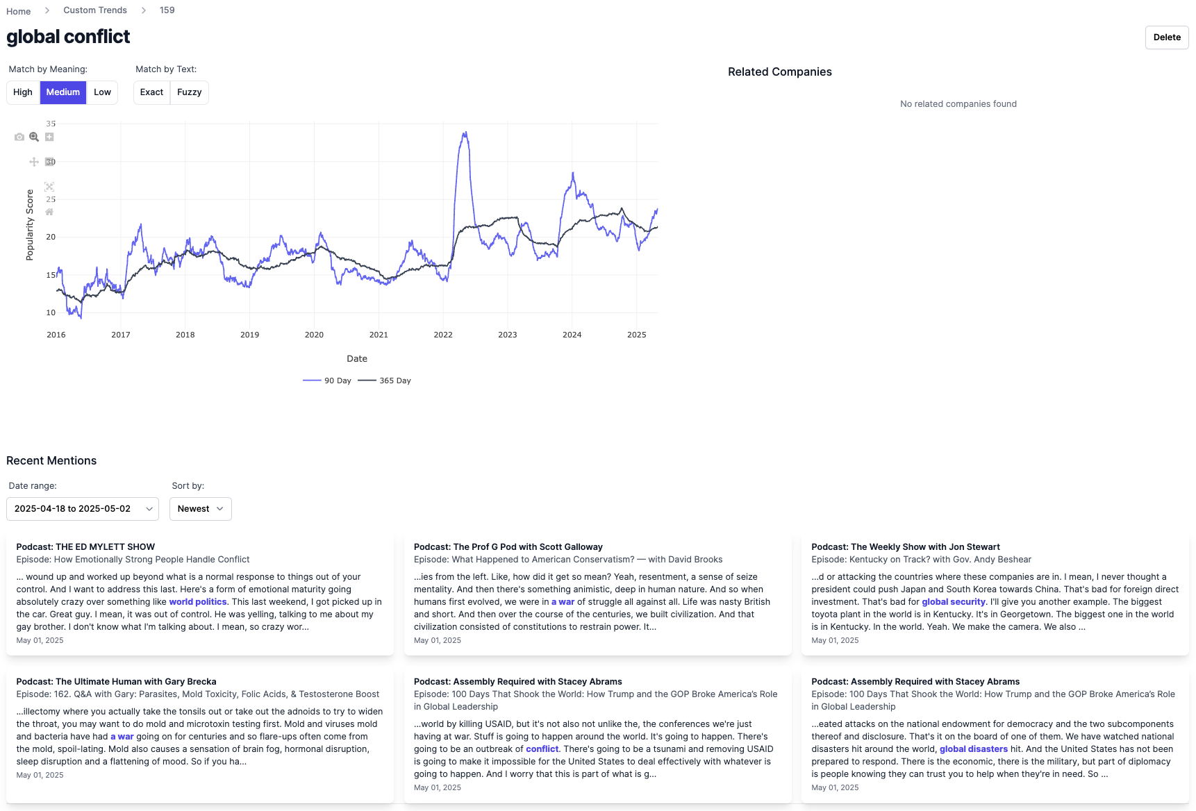
Note the spikes in 90 day popularity preceding and during the onset of the Russia-Ukraine war, US tariffs, etc.
3. Analysis: Custom Hivemind Factor Correlations with Forward VIX
Let's analyze the correlations between our Hivemind-generated factors and forward 10-day changes in VIX from 2016 to present. These raw correlations and associated p-values should help us identify and validate that our factors are leading indicators of volatility spikes.
While we will use 10, 15, 20, 25, and 30 day (backwards-looking) factor growth for making forward VIX growth predictions, we only show 20 day (backwards-looking) factor growth below to save space.
| Factor Δ | Spearman Corr (P-Value) | Pearson Corr (P-Value) |
|---|---|---|
| 20d_growth_global conflict_90d | 0.06 (0.00) | 0.08 (0.00) |
| 20d_growth_unemployment_90d | 0.06 (0.01) | 0.09 (0.00) |
| 20d_growth_market_crash_90d | 0.05 (0.02) | 0.09 (0.00) |
| 20d_growth_anxiety_90d | 0.02 (0.38) | 0.06 (0.00) |
Anxiety levels are not strongly rank-order (Spearman) correlated on their own with forward changes to VIX. However, given this factor is intuitive and has a high Pearson correlation, we are going to keep it; it will help our non-linear modelling efforts later in this article.
Let's also quickly confirm our delta Hivemind factors aren't too (Pearson) correlated with each other:
| Factor Δ | Anxiety | Unemployment | Market Crash | Global Conflict |
|---|---|---|---|---|
| 20d_growth_anxiety_90d | 1.00 | 0.21 | 0.29 | 0.02 |
| 20d_growth_unemployment_90d | 0.21 | 1.00 | 0.11 | (0.07) |
| 20d_growth_market crash_90d | 0.29 | 0.11 | 1.00 | 0.03 |
| 20d_growth_global conflict_90d | 0.02 | (0.07) | 0.03 | 1.00 |
They are not, and as such should all be additive to our forecasts. Excellent!
4. Analysis: Previous VIX Momentum Correlations with Forward VIX
Often, previous changes in the target variable itself (i.e. momentum factors) are correlated with forward changes. Given the VIX is mean-reverting, sign-flipped previous changes should be correlated. Let's explore that below.
| Factor Δ | Spearman Corr (P-Value) | Pearson Corr (P-Value) |
|---|---|---|
| prev_100d_growth_VIX_sign_flipped | 0.25 (0.00) | 0.18 (0.00) |
| prev_30d_growth_VIX_sign_flipped | 0.28 (0.01) | 0.18 (0.00) |
| prev_10d_growth_VIX_sign_flipped | 0.21 (0.02) | 0.17 (0.00) |
They are, and as such should all be additive to our forecasts. Great!
5. Analysis: Composite Hivemind Factor Correlations with Forward VIX
Next, let's create composite factors using weighted combinations of our delta factors over a mix of growth horizons. They should provide smoother and more stable signals.
| Factor Δ | Spearman Corr (P-Value) | Pearson Corr (P-Value) |
|---|---|---|
| growth_composite_90d | 0.34 (0.00) | 0.27 (0.00) |
| growth_composite_global conflict_90d | 0.07 (0.00) | 0.08 (0.00) |
| growth_composite_market_crash_90d | 0.05 (0.02) | 0.09 (0.00) |
| growth_composite_unemployment_90d | 0.05 (0.02) | 0.10 (0.00) |
| growth_composite_anxiety_90d | 0.02 (0.29) | 0.06 (0.00) |
6. Analysis: ML For VIX Forecasts
Using all of the factors we've created thus far, let's use XGBoost to forecast our target variable: 10-day (forward) changes in VIX.
We'll use the oldest 75% of dates as our training set and newest 25% of dates (less a 10 day gap to avoid lookahead) as our test set.
6.1 Train XGBoost Model to Predict Forward VIX Changes
import xgboost as xgb

import numpy as np
np.random.seed(42)

TARGET = 'fwd_10d_growth_VIX'

# Copy the original time-series factor DataFrame for ML use
ml_df = merged_df.copy()

# Drop rows with NaNs
ml_df = ml_df.dropna()

# Determine split index (75% train, 25% test)
split_idx = int(len(ml_df) * 0.75)

# Train / test split (df already sorted oldest -> newest)
train = ml_df.iloc[:split_idx]
test = ml_df.iloc[split_idx + 10:]

X_train = train.drop(columns=[col for col in ml_df.columns if "fwd" in col])
y_train = train[TARGET]
X_test = test.drop(columns=[col for col in ml_df.columns if "fwd" in col])
y_test = test[TARGET]

# Train model
model = xgb.XGBRegressor(
    n_estimators=1000,
    max_depth=4,
    learning_rate=0.003,
    subsample=0.6,
    colsample_bytree=0.8,
    colsample_bylevel=0.8
)
model.fit(X_train, y_train)

# Predict
y_pred = model.predict(X_test)
6.2 Visualize Predictions vs Actuals
It's often easier to see performance, so let's visualize how we did below.
Evolution:
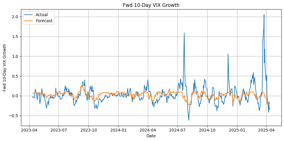
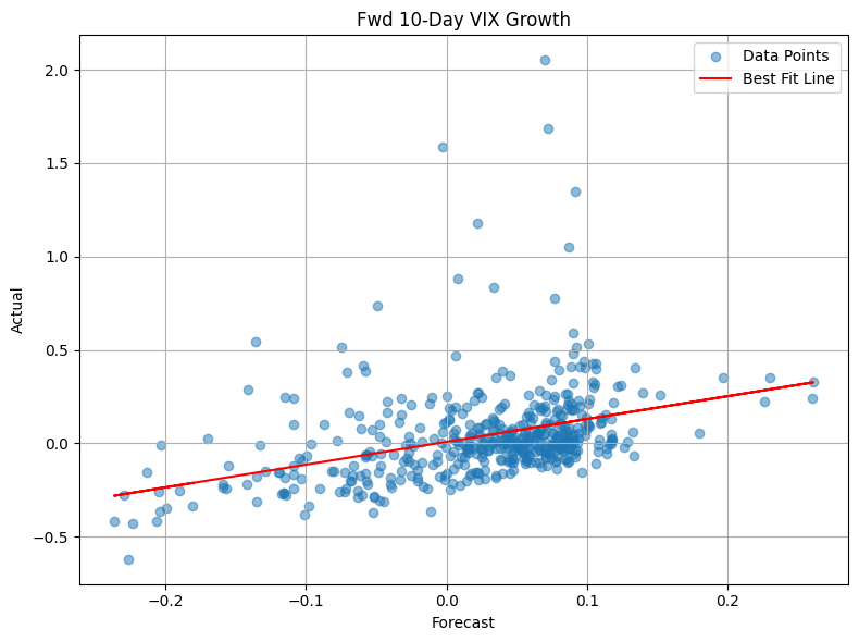
Scatterplot:

Looks like we've done fairly well! Let's quantify our performance next.
6.3 Quantify Performance
Running the below code, we get:
- 63.8% hit rate (directional accuracy)
- 13.2% R² score (explained variance)
- 0.37 Pearson correlation
- 0.46 Spearman correlation
import numpy as np
from scipy.stats import spearmanr, pearsonr
from sklearn.metrics import r2_score

y_hat = y_pred
y = y_test.values

# Hit rate (directional accuracy)
hit_rate = np.mean(np.sign(y_hat) == np.sign(y))
print(f"Hit rate: {hit_rate:.2%}")

# Explained variance (R²)
r2 = r2_score(y, y_hat)
print(f"R² score (change in VIX): {r2:.4f}")

# Correlations
pearson_corr, pearson_pval = pearsonr(y_hat, y)
spearman_corr, spearman_pval = spearmanr(y_hat, y)
print(f"Pearson correlation: {pearson_corr:.4f} (p-value: {pearson_pval:.4g})")
print(f"Spearman correlation: {spearman_corr:.4f} (p-value: {spearman_pval:.4g})")
7. Suggested Improvements
- Add more features / factors: market-based, macro / economic indicators, VIX term structure, alternative data, Hivemind sentiment factors, etc.
- Train ML model on a rolling-window basis with walk-forward validation
- Ensemble predictions across models trained at different time horizons
- Grid-search hyperparameters
- Try other ML models
- Run SHAP to better understand forecast drivers and remove features that aren't sufficiently additive / helpful to reduce noise
8. Why We Built Hivemind
Imagine knowing what consensus views were, and how they were evolving, about anything, throughout time.
Creating accurate forecasts for anything would be easy with perfect access to features / factors representing aggregate popularity and sentiment for anything. The market, after all, is just aggregate sentiment.
However, this aforementioned humankind popularity and sentiment factor forge doesn't exist, and so creating accurate forecasts is hard.
We (very naively) thought we could create a tool using new developments in AI that allowed anyone to create well-founded time-series factors for anything in one line of code.
We were wrong. For several months and several disappointing Hivemind iterations.
But recently, after lots of improvements to our AI, software, and data architecture, Hivemind has started to work. We've built a humankind popularity and sentiment factor forge for any time-series factor you can imagine!
Right now, it's predominantly based on discussion from top US podcasts, but we will continue to add new (quality, non-AI generated) media sources to strengthen the Hivemind.
While our popularity factor forge is live today (and was used to create forecasts in this article), our sentiment factor forge is currently being finalized; expect to see it in the next couple of weeks!
We built Hivemind to allow anyone to create any popularity or sentiment time-series factor in one line of code; we're excited to see what you do with it!
9. Closing / Contact Info
Using ForecastOS Hivemind, we easily created custom factors and an associated model that predicts 10-trading-day forward changes to VIX during our test period (last ~2 years) with:
- 63.8% hit rate (directional accuracy),
- 13.2% R² score (explained variance),
- 0.37 Pearson correlation, and
- 0.46 Spearman correlation.
If you’re interested in using Hivemind for your own research / to create your own custom factors, drop us a line: trialaccess @ forecastos.com.
Notebook and code used for this article available to ForecastOS clients @ app.forecastos.com/research